7. ATAC-seq : Footprinting analysis using TOBIAS

Tn5 bias correction

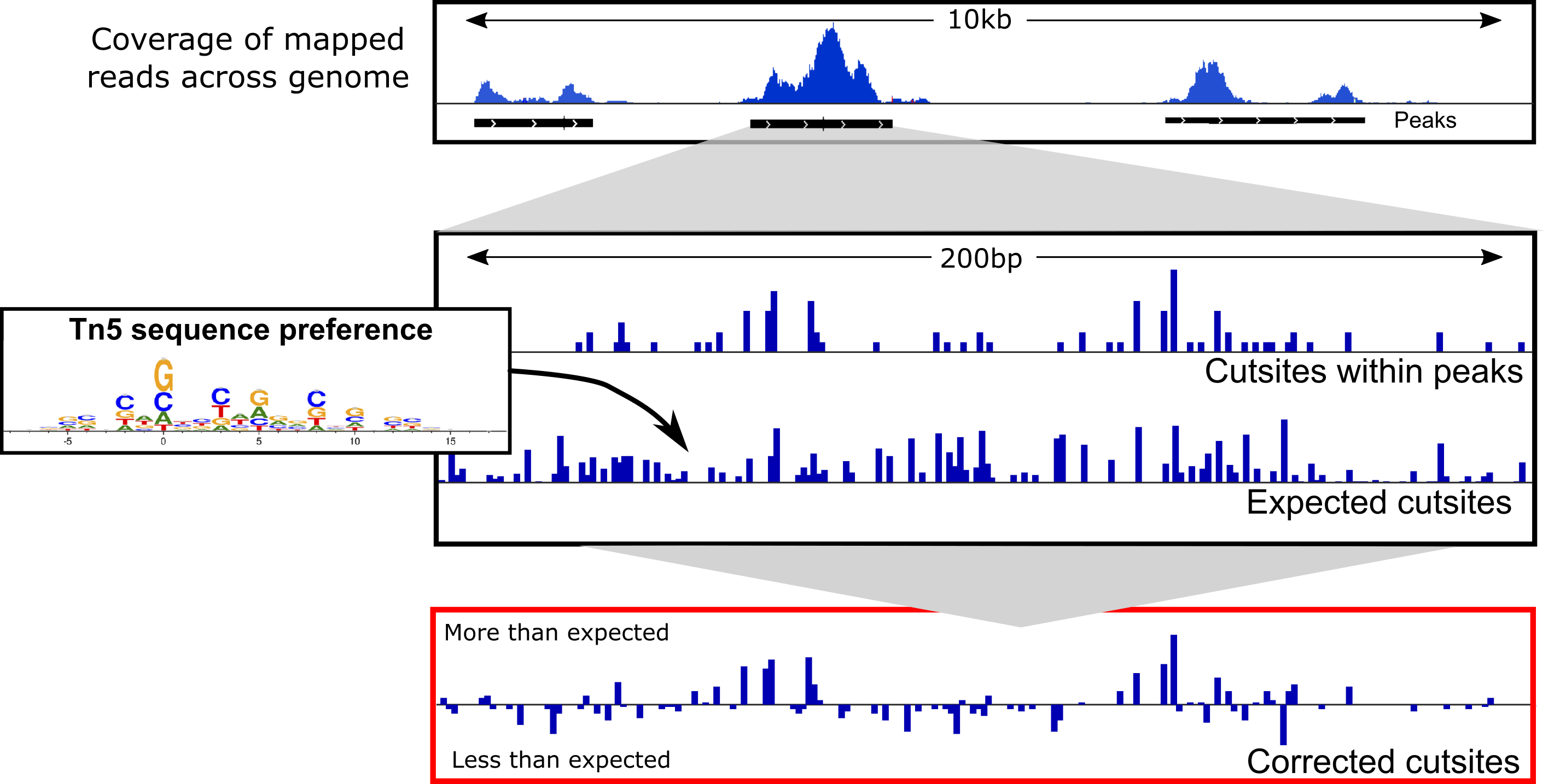Figure taken from TOBIAS

The function ATACorrect from TOBIAS is used for the following reasons -

• During ATACseq libtrary preparation, the Tn5 transposase binds to the open chromatin as a dimer and inserts two adapters separated by 9 bps. This has no major effect in peak calling, however, for footprinting analysis, the + and - strand are shifted by +4 bps and −5 bps repectively see this and this. Doing so helps identify the center of the Tn5 binding.

• Though we expect Tn5 to bind randomly in open regions, in reality, Tn5 has a binding bias towards specific sequence. Thus, within a given open chromatin region, it's more likely to find the Tn5 cutsites over these specific sequences. This inherent bias needs to be corrected to identify the cutsites accurately. The function calculates the difference between the observed vs expected cutsites to correct for this bias.

cd

mkdir -p analysis/Footprint

##################################################
#### THIS IS A LENGTHY PROCESS, DO NOT RUN IT ####
##################################################

TOBIAS ATACorrect \
--bam data/processed/ATACseq/Bowtie2/ATAC_REP1_aligned_filt_sort_nodup.bam  \
--genome data/ext_data/genome.fa \
--peaks analysis/MACS2/ATAC/ATAC-Rep1_peaks.narrowPeak \
--cores 3 \
--outdir analysis/Footprint/

Footprinting scores

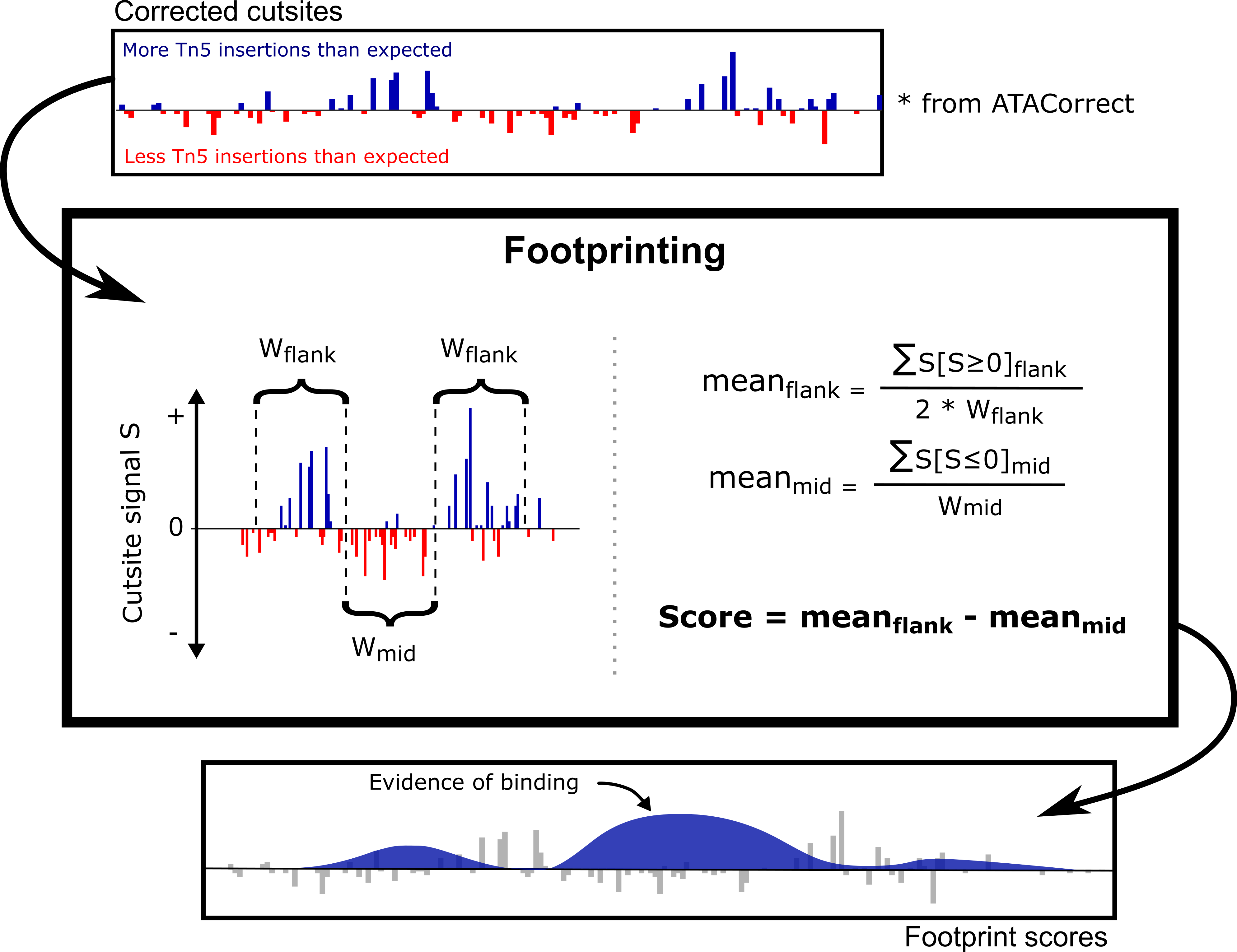Figure taken from TOBIAS

Using the Tn5 bias corrected signals, this function estimates the footprints (i.e putative TF binding sites) within peak regions by identifying regions with depleted cutsite signal and flanked by high cutsite signal. Such a signal pattern indicates regions of TF binding.

cd

##################################################
#### THIS IS A LENGTHY PROCESS, DO NOT RUN IT ####
##################################################

TOBIAS ScoreBigWig \
--signal analysis/Footprint/ATAC_REP1_aligned_filt_sort_nodup_corrected.bw \
--regions analysis/MACS2/ATAC/ATAC-Rep1_peaks.narrowPeak \
--cores 3 \
--output analysis/Footprint/ATAC_footprints.bw 

Transcription factor binding prediction

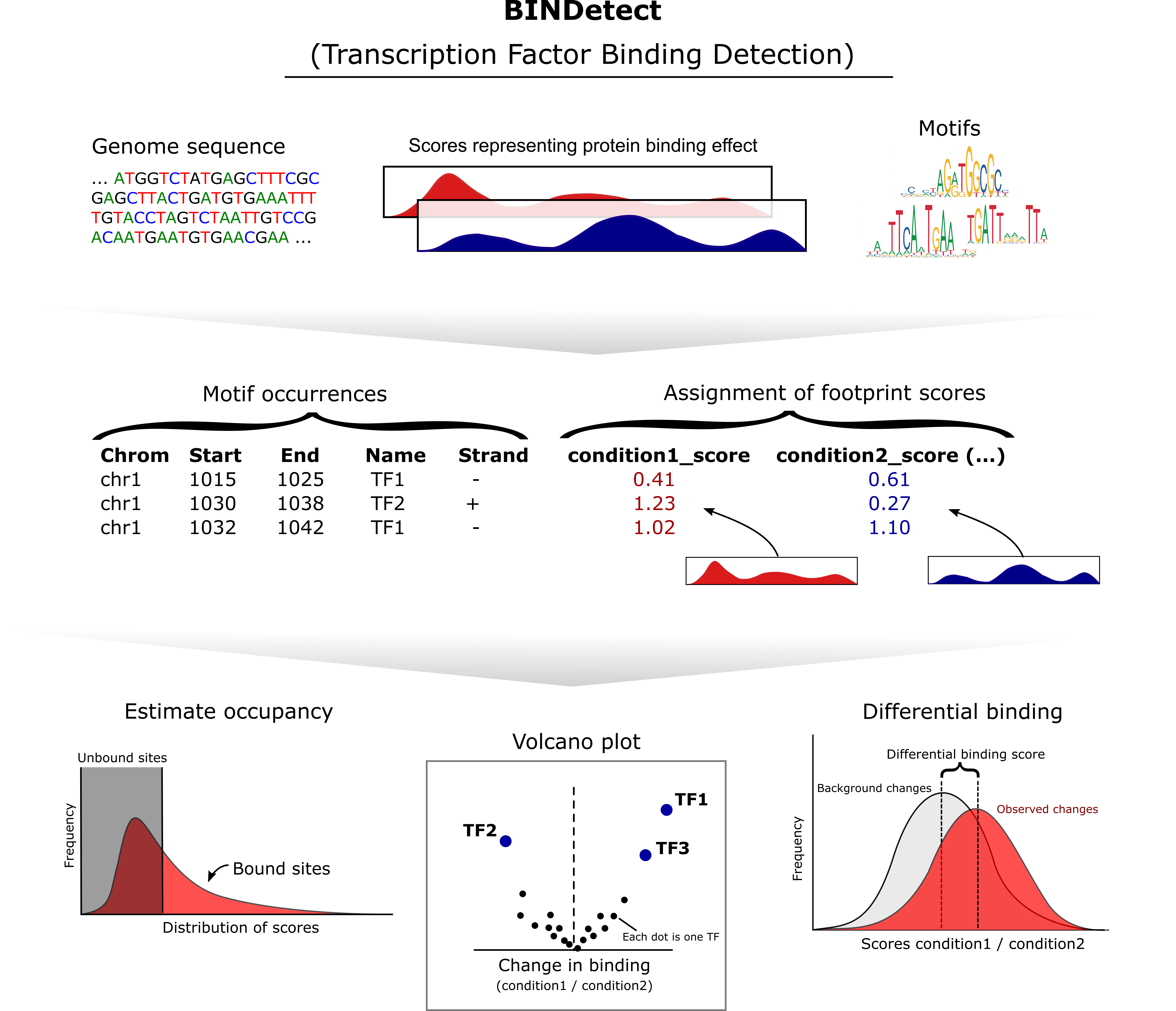Figure taken from TOBIAS

Once the footprint regions are identified, one could look at the sequence at those regions and compare that with the TF binding motif sequence to estimate the TF binding propensity at the footprint regions. TF binding motifs are provided in standard JASPAR format.

This step takes about ~7 minutes

cd

mkdir -p analysis/Footprint/BINDdetect

TOBIAS BINDetect \
--motifs data/ext_data/motifs.jaspar \
--signals data/processed/ATACseq/Footprint/ATAC_footprints.bw  \
--genome data/ext_data/genome.fa \
--peaks analysis/MACS2/ATAC/ATAC-Rep1_peaks.narrowPeak \
--cores 3 \
--outdir analysis/Footprint/BINDdetect

Using Cyberduck, go to the folder generated (analysis/Footprint/BINDdetect). Check one of the folders (for exampe for CTCF):

• open the png file: what does it show?
• open the beds folder: do you understand what the content represents?

Task - integrative analysis

Using Cyberduck download these files to you local machine -

CTCF

1. analysis/MACS2/CTCF/CTCF_peaks.narrowPeak
2. analysis/bigwig/ChIP/CTCF_ses_subtract.bw

ATAC

3. analysis/MACS2/ATAC/ATAC-Rep1_peaks.narrowPeak
4. data/processed/ATAC/bigwig/ATAC_REP1.bw

Footprints

5. analysis/Footprint/BINDdetect/CTCF_MA0139.1/beds/CTCF_MA0139.1_ATAC_footprints_bound.bed
6. analysis/Footprint/BINDdetect/KLF4_MA0039.4/beds/KLF4_MA0039.4_ATAC_footprints_bound.bed

Load these track in IGV and try to answer the following -

Don't forget to change the genome to hg38 by clicking at Genome. Next, click on Tracks to load these files from your local computer

You have been working with HCT116 cell-line (colon cancer), here is a list of genes implicated in colon cancer. Try looking at genes like APC, CCND1, YTHDC2, ELL2 etc

1. Do the .bigwig peaks (SES) and the MACS2 called .narrowPeak correspond in CTCF
2. Do the .bigwig peaks (bamCompare) and the MACS2 called .narrowPeak correspond in ATAC
3. Are there region where CTCF and ATAC peaks overlap
4. Can you find CTCF/ATAC overlapping peak regions at the promoter regions or enhancer regions of these genes
5. Do TF binding site for CTCF and KLF4 overlap ?

Overlap between CTCF Chipseq and CTCF footprinting

The obvious question we have is how well does the CTCF ChIPseq peaks correspond to the CTCF binding sites predicted from the footprinting analysis on ATACseq data.

cd

/usr/bin/R

# Now you are in the R console

library(rtracklayer)

CTCFchip = import("/home/user22/analysis/MACS2/CTCF/CTCF_peaks.narrowPeak")

CTCFfoot = read.table("/home/user22/analysis/Footprint/BINDdetect/CTCF_MA0139.1/beds/CTCF_MA0139.1_ATAC_footprints_bound.bed", stringsAsFactors=F, sep="\t")[,1:4]
colnames(CTCFfoot) = c('chr','start','end','name')
CTCFfoot = makeGRangesFromDataFrame(CTCFfoot)

# How many binding sites called ?
length(CTCFfoot)

# How many peaks in the CTCF ChIPseq ?
length(CTCFchip)

# Overlap analysis
CTCFchip_peak_count = length(CTCFchip)
overlap_count = sum(CTCFchip %over% CTCFfoot)

length(overlap_count)

overlap_count/CTCFchip_peak_count * 100

# 20.51207

Given the % overlap you calculated.

• What do you think ? Is the overlap high/low ? Is this expected ?
• In the overlap analysis above we answer - How many of the CTCF ChIPseq peaks are present in CTCF footprints ? Now try answering the opposite - Of all the predicted CTCF footprints, what % of those were overlapping with CTCF Chipseq peaks.
• Biologically speaking why these numbers differ ? Hint: Think of how the regulatory landscape changes by condition/environment etc